© 2013 Oceanic Imaging Consultants, Inc.

Service + Software for Seafloor Mapping

Seafloor mapping is largely a matter of measuring depth. Prior to the First World War, the depth of the oceans was usually measured by lead lining. This involved lowering a chunk of lead (usually a cannonball) on a very long piano wire to the bottom of the sea. In 1826, Daniel Colladon measured the speed of sound in the waters of Lake Geneva, Switzerland. This experiment was one of many steps toward the creation of sonar. However, using sonar remained in the experimental stage for another 90 years, and sailors continued to make their measurements the old fashioned way.
The First World War changed all this when Germany put submarines into action against allied ships. The ships had no way of seeing the submarines coming. The U.S. War Department asked scientists what could be done about this problem. The resulting war effort produced (a) government funding of research, and (b) anti-submarine warfare, which resulted in the accelerated development of underwater technology. Submarines also benefited from echo technology when sound sources were installed on the submarines for both echolocation and Morse code.
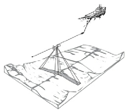
After using underwater sound technology for measuring the proximity to the shore and other ships, researchers soon realized that if the sound device was pointed down at the seafloor, the depth could be accurately determined. Early “echo sounders”, as they were called, had very poor directivity and relied on the assumption that the echoes were coming from directly beneath the vessel. The included angle (cone of the beam pattern out to the 3 dB down point) was about 60 degrees. This was a poor assumption if there was any shape to the seafloor below, but it was easier than the old lead line method and could be carried out while under way(see Figure 1).
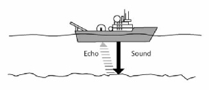
Marine Geology, which was a relatively new science at the time, also helped with the development of sonar (see Figure 2).
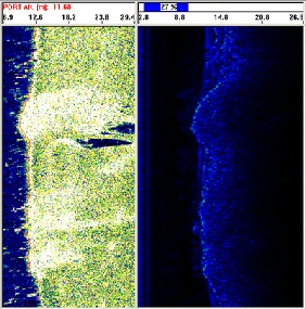
Marine Geologists found that if you put enough energy into the “ping” you could get echoes from the layers of sediments and rocks beneath the bottom profile, and called this the “sub-bottom profile” (Figure 2). By recording the amplitude of the backscatter energy as a function of time and making some assumptions about sound velocity in the water (1500 m/sec) and the rocks (faster than 1500 m/sec), marine geologists could convert this data into water depth and rock layer thickness. By pinging continuously, driving the boat in straight lines, and laying all the ping records next to each other, they got an image, which looked like a vertical profile through the water column and sub-bottom. Dark reflectors correspond to scattered energy from point scatterers or layer transitions, termed changes in acoustic impedance (density * compressional wave sound velocity in the upper layer divided by the same for the lower layer). (See Figure 3).
Brief History of Sonar Development (page 1 of 4)
Figure 1. Typical echo sounder’s dynamics
Figure 2. A comparison of bottom tracking and sub-bottom profile, from SIS-1000 data
Figure 3. Geometry of a typical sidescan sonar